Introduction
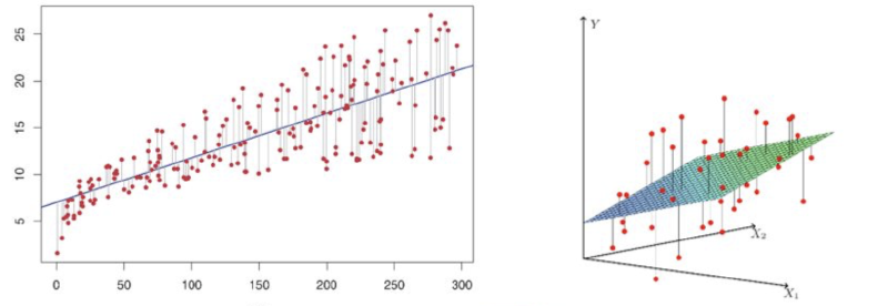
The goal is to find the linear model $y = \beta_0 + \beta_1 x$ such that the sum of squared errors between the predicted values and the actual data is minimized.
Linear Model
The form of the linear model is:
$$ y_i = \beta_0 + \beta_1 x_i + \epsilon_i $$
where $y_i$ is the observed value, $x_i$ is the independent variable, $\beta_0$ is the intercept, $\beta_1$ is the slope, and $\epsilon_i$ is the error term.
We wish to find $\beta_0$ and $\beta_1$ such that the predicted values $\hat{y}_i = \beta_0 + \beta_1 x_i$ minimize the sum of squared errors between $\hat{y}_i$ and the observed values $y_i$.
Design Matrix and Observation Vector
To make the problem more convenient, we represent it using vectors and matrices.
Design Matrix
Define the design matrix $\mathbf{X}$ as:
$$ \mathbf{X} = \begin{bmatrix} 1 & 1 \newline 1 & 2 \newline 1 & 3 \newline 1 & 4 \end{bmatrix} $$
The first column contains only 1s, representing the constant term $\beta_0$, and the second column contains the values of the independent variable $x_i$.
Observation Vector
Define the observation vector $\mathbf{y}$ as:
$$ \mathbf{y} = \begin{bmatrix} 2 \newline 3 \newline 5 \newline 7 \end{bmatrix} $$
This vector contains all the observed values $y_i$.
Parameter Vector
Define the parameter vector $\boldsymbol{\beta} = \begin{bmatrix} \beta_0 \newline \beta_1 \end{bmatrix}$.
Sum of Squared Errors Objective Function
In regression, our goal is to find the parameters $\boldsymbol{\beta}$ such that the predicted values $\hat{\mathbf{y}} = \mathbf{X} \boldsymbol{\beta}$ are as close as possible to the observed values $\mathbf{y}$, by minimizing the sum of squared errors (SSE):
$$ S(\beta_0, \beta_1) = \sum_{i=1}^n (y_i - \hat{y}_i)^2 = (\mathbf{y} - \mathbf{X} \boldsymbol{\beta})^T (\mathbf{y} - \mathbf{X} \boldsymbol{\beta}) $$
Deriving the Normal Equation
The key idea of least squares is to find $\boldsymbol{\beta}$ such that the residual $\mathbf{y} - \mathbf{X} \boldsymbol{\beta}$ is minimized. Geometrically, this means that the residual should be orthogonal to the column space of the design matrix $\mathbf{X}$, which leads to the normal equation:
$$ \mathbf{X}^T (\mathbf{y} - \mathbf{X} \hat{\boldsymbol{\beta}}) = 0 $$
Expanding this:
$$ \mathbf{X}^T \mathbf{y} = \mathbf{X}^T \mathbf{X} \hat{\boldsymbol{\beta}} $$
This is the normal equation, which can be solved to find the least squares estimate $\hat{\boldsymbol{\beta}}$.
Solving the Normal Equation
Now, let’s compute the parts of the normal equation.
Compute $\mathbf{X}^T \mathbf{X}$
$$ \mathbf{X}^T \mathbf{X} = \begin{bmatrix} 1 & 1 & 1 & 1 \newline 1 & 2 & 3 & 4 \end{bmatrix} \begin{bmatrix} 1 & 1 \newline 1 & 2 \newline 1 & 3 \newline 1 & 4 \end{bmatrix} = \begin{bmatrix} 4 & 10 \newline 10 & 30 \end{bmatrix} $$
Compute $\mathbf{X}^T \mathbf{y}$
$$ \mathbf{X}^T \mathbf{y} = \begin{bmatrix} 1 & 1 & 1 & 1 \newline 1 & 2 & 3 & 4 \end{bmatrix} \begin{bmatrix} 2 \newline 3 \newline 5 \newline 7 \end{bmatrix} = \begin{bmatrix} 17 \newline 50 \end{bmatrix} $$
Solve the Normal Equation
Now we solve the normal equation:
$$ \begin{bmatrix} 4 & 10 \newline 10 & 30 \end{bmatrix} \hat{\boldsymbol{\beta}} = \begin{bmatrix} 17 \newline 50 \end{bmatrix} $$
To solve this, we first compute the inverse of $\mathbf{X}^T \mathbf{X}$:
$$ (\mathbf{X}^T \mathbf{X})^{-1} = \frac{1}{(4)(30) - (10)(10)} \begin{bmatrix} 30 & -10 \newline -10 & 4 \end{bmatrix} = \frac{1}{20} \begin{bmatrix} 30 & -10 \newline -10 & 4 \end{bmatrix} $$
Next, we compute $\hat{\boldsymbol{\beta}}$:
$$ \hat{\boldsymbol{\beta}} = (\mathbf{X}^T \mathbf{X})^{-1} \mathbf{X}^T \mathbf{y} $$
$$ \hat{\boldsymbol{\beta}} = \frac{1}{20} \begin{bmatrix} 30 & -10 \newline -10 & 4 \end{bmatrix} \begin{bmatrix} 17 \newline 50 \end{bmatrix} = \frac{1}{20} \begin{bmatrix} (30)(17) + (-10)(50) \newline (-10)(17) + (4)(50) \end{bmatrix} $$
$$ \hat{\boldsymbol{\beta}} = \frac{1}{20} \begin{bmatrix} 510 - 500 \newline -170 + 200 \end{bmatrix} = \frac{1}{20} \begin{bmatrix} 10 \newline 30 \end{bmatrix} = \begin{bmatrix} 0.5 \newline 1.5 \end{bmatrix} $$
Least Squares Estimate
By solving the normal equation, we find $\hat{\beta}_0 = 0.5$ and $\hat{\beta}_1 = 1.5$. Thus, the regression model is:
$$ \hat{y} = 0.5 + 1.5x $$
Conclusion
Using the projection approach, we see that the least squares estimate is the projection of the observation vector $\mathbf{y}$ onto the space spanned by the columns of the design matrix $\mathbf{X}$. By solving the normal equation, we found the parameters $\hat{\beta}_0 = 0.5$ and $\hat{\beta}_1 = 1.5$, which minimize the sum of squared errors.
