YOPO – You Only Pick Once
1 Objective
The aim is to implement a simple yet effective object tracking algorithm that does not rely on neural networks. We are given several frames from a video of a street, the task is to first pick a car from the first frame, then track the car in the subsequent frames.
2 Ideas
There are three problems to solve in this task:
2.1 Object Changing
Problem: The shape and color of the object may change over time. If we use a fixed template (from the first frame) to search for the object in all subsequent frames, the matching score will drop significantly and eventually fail to capture the object.
Solution: Update the template (kernel). Whenever we find the object with a high confidence, we update the template (also called the kernel) with the newly found object. Therefore making the kernel adaptive to the changing object.
2.2 High Computational Cost
Problem: If we search for the object in the whole image, the computational cost is exteremely high.
Solution: Use prior knowledge. In real-world streets, the position (or velocity) and the shape of the car change extremely slowly given a high frame rate. Therefore, we could potentially use the history of the car to predict its position in the next frame, and only search for the car in a small region around the predicted position.
2.3 Finding Matching Score
Problem: How do you find a “confidence” matching score between the kernel and a candidate region? Using inner products?
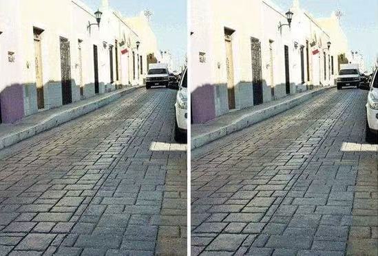
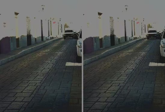
Solution: Normalized Cross-Correlation (NCC). Inner product is almost the answer except that the outcome is sensitive to brightness. For example, the inner product between the two images in Figure 1 and Figure 2 is \(2706529500.0\) and \(770488300.0\) respectively, though they look exactly the same respectively.
Therefore, we need to normalize the inner product: Suppose \(T\), \(W\) are two images of size \(h\times w\). We consider them as a long vector in \(\mathbb{R}^{hw}\) instead of matrices. First of all, they are “above the horizon” (non-negative), so we subtract the mean value from each image to make them “zero-mean”:
\[ \begin{aligned} T &\to \tilde{T} = T - \mu_T \quad \left(\mu_T = \frac{1}{hw} \sum_{i} T_i\right) \\ W &\to \tilde{W} = W - \mu_W \quad \left(\mu_W = \frac{1}{hw} \sum_{i} W_i\right) \end{aligned} \]
Then, define the NCC (normalized cross-correlation) between \(T\) and \(W\) as the \(\cos \angle (\tilde{T}, \tilde{W})\), i.e.,
\[ \begin{aligned} \text{NCC}(T, W) :&= \frac{\langle \tilde{T}, \tilde{W} \rangle}{\|\tilde{T}\|_2 \|\tilde{W}\|_2} \\ &= \frac{\sum_i (T_i - \mu_T)(W_i - \mu_W)}{\sqrt{\sum_i (T_i - \mu_T)^2} \sqrt{\sum_i (W_i - \mu_W)^2}} \\ &\in [-1, 1] \end{aligned} \tag{1}\]
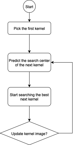
3 Methodology
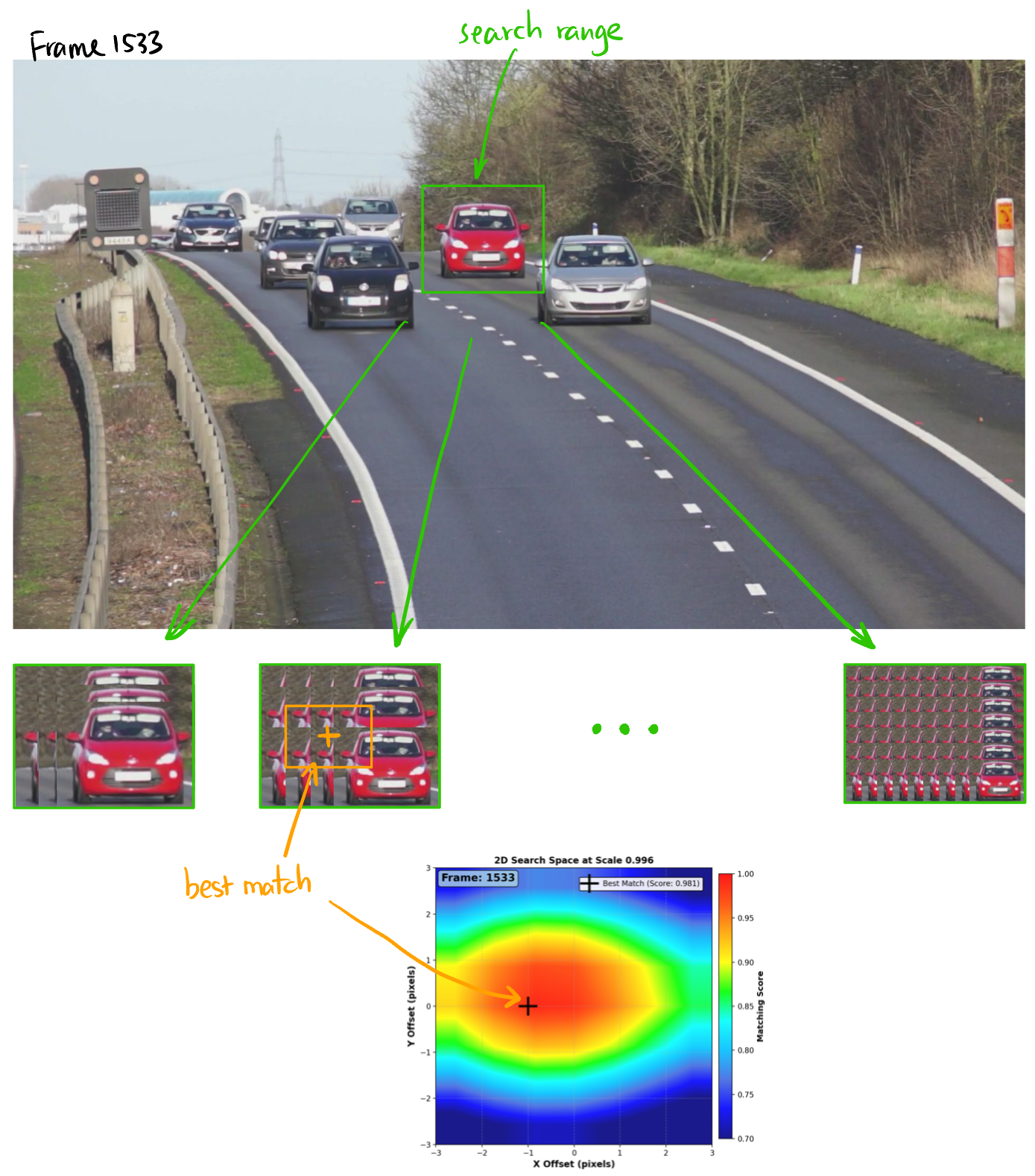
The overall algorithm is summarized in the flowchart Figure 3, which is explained in detail in the following sections.
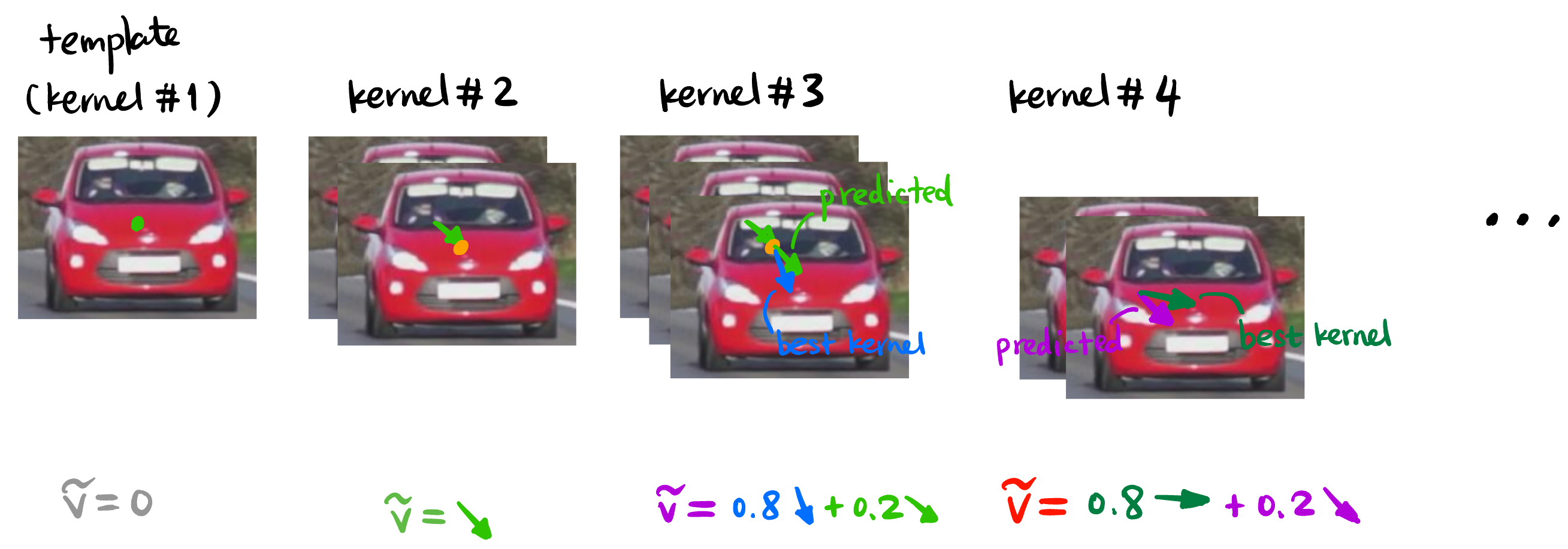
3.1 Predict the Next Search Window Center
First frame: Since the object’s speed and direction are initially unknown, we manually select the object in the first frame and use its center as the initial search location.
Second frame: Once we identify the object in the second frame (via Section 3.2), we now have two locations, which allows us to compute an initial velocity vector \(v_1\) (the green arrow in Figure 4).
Third frame: We directly use \(v_1\) to predict the center of the search area in the third frame. After finding a best kernel in the third frame, we have another velocity vector \(v_2\). We then average \(v_1\) and \(v_2\) to get a more stable velocity estimate: \[ v_3 \approx \alpha v_2 + (1-\alpha) v_1 \quad (\alpha \in [0,1]) \]
Subsequent frames: Use \(v_{n-1}\) to predict the center of the search area in the \((n+1)\)-th frame. After finding a best kernel in the \((n+1)\)-th frame, we have another velocity vector \(v_n\). We then average \(v_n\) and \(v_{n-1}\) to get a more stable velocity estimate: \[ v_{n+1} \approx \alpha v_{n} + (1-\alpha) v_{n-1} \quad (\alpha \in [0,1]) \]
3.2 Local Search with NCC and Kernel Resizing
This module receives the predicted search center from Section 3.1 and the current kernel image.
Step 1: Local search window We define a search window of \(\pm 3\) pixels vertically and horizontally from the predicted center. For each candidate region, we compute the NCC (Normalized Cross-Correlation) score defined in Equation 1.
Step 2: Kernel resizing Since the object (a car) may change in size as it moves closer or farther from the camera, we also resize the kernel (both enlarged and shrunk) and repeat the NCC search at each scale.
Step 3: Best match selection We now have three sets of NCC scores (one per kernel scale). We select the candidate with the maximum NCC score across all scales, and define that as the detection result for the current frame.
Step 4: Handoff to next stage The matched region’s location is used to update the predicted trajectory, and the cropped image may or may not be used as the new kernel — this decision is handled in the next module in Section 3.3.
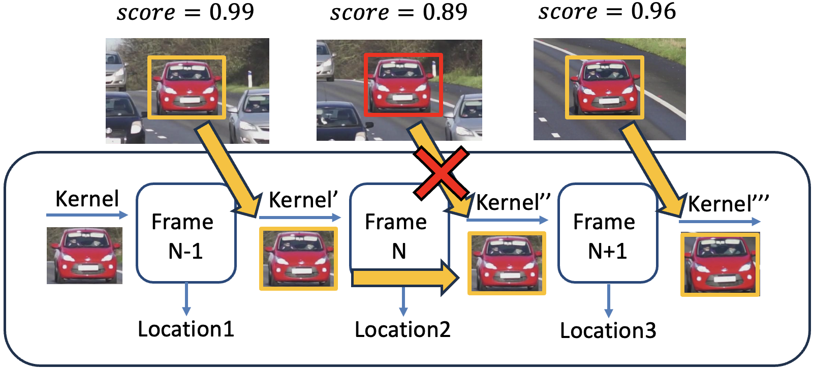
3.3 Kernel Updating Rule
In this module, we address the question: Should we update the kernel image every frame?
Problem with naïve updates: Simply picking the top-matching region as the new kernel in every frame might lead to error accumulation, especially when the background changes or the match is unreliable.
Our key principles are:
- Always update the kernel’s location, because tracking requires positional accuracy.
- Only update the kernel’s image if the match quality is sufficiently high.
- Threshold-based strategy:
- Define a threshold for NCC similarity (e.g., \(\text{NCC}_{\text{thres}} = 0.94\)).
- If the current best match has a \(\text{NCC} > 0.94\), it means the match is strong — we update both kernel location and image.
- If \(\text{NCC} < 0.94\), the match might be unreliable (e.g., due to a temporary background obstruction like a white pole as shown in Figure 6). In this case, we only update the position, and retain the previous kernel image for consistency.
- Threshold-based strategy:
- Example (Figure 6):
- Frame 1: \(\text{NCC} = 0.99 > \text{NCC}_{\text{thres}}\): update both position and image.
- Frame 2: \(\text{NCC} = 0.89 < \text{NCC}_{\text{thres}}\): update only position.
- Frame 3: \(\text{NCC} = 0.96 > \text{NCC}_{\text{thres}}\): update both.
This adaptive mechanism avoids abrupt kernel drift and helps maintain robustness in challenging tracking conditions.
4 Results
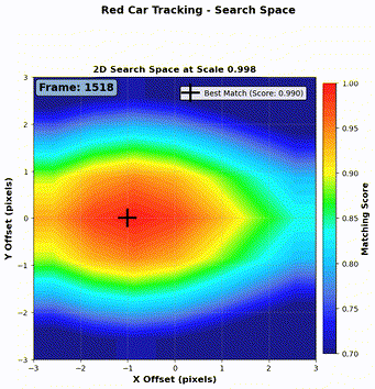
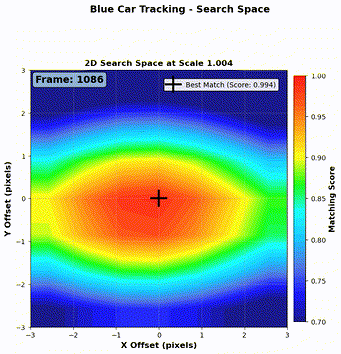
As shown in Figure 7 and Figure 8, our algorithm successfully tracks both a red car and a blue car throughout the video sequence.
5 Future Work
Blocking views: Our current method struggles when the target is briefly occluded (e.g., by other vehicles or obstacles). Future work could integrate motion prediction with re-identification techniques to maintain tracking through occlusion.
Cumulative error: Due to the iterative nature of kernel updates and position prediction, small errors may accumulate over time. Incorporating global correction mechanisms (e.g., periodic full-frame verification) could help mitigate this drift.